Visualization of MLP weights on MNIST

Sometimes looking at the learned coefficients of a neural network can provide insight into the learning behavior. For example if weights look unstructured, maybe some were not used at all, or if very large coefficients exist, maybe regularization was too low or the learning rate too high.

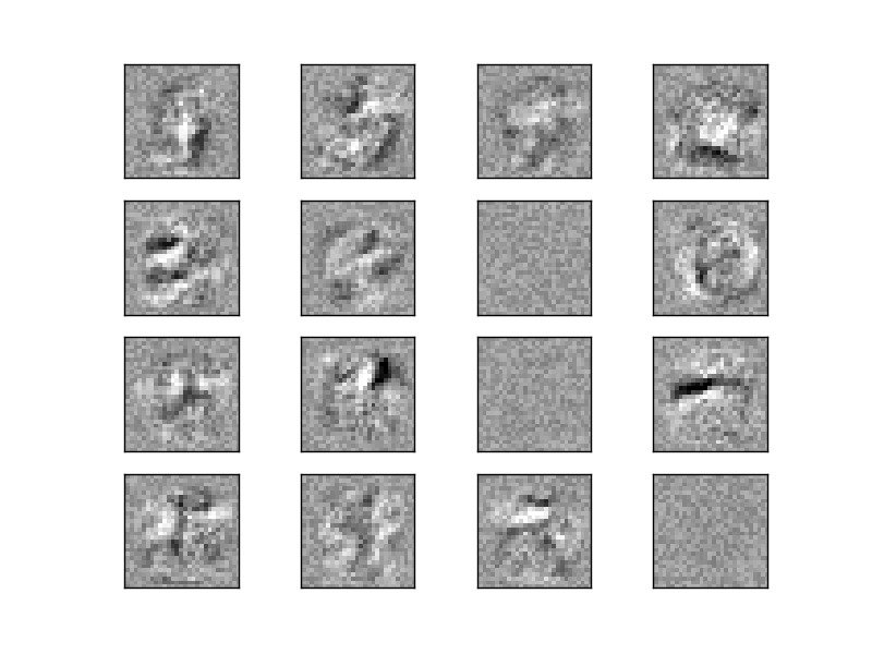
This example shows how to plot some of the first layer weights in a MLPClassifier trained on the MNIST dataset.

The input data consists of 28x28 pixel handwritten digits, leading to 784 features in the dataset. Therefore the first layer weight matrix have the shape (784, hidden_layer_sizes[0]). We can therefore visualize a single column of the weight matrix as a 28x28 pixel image.

To make the example run faster, we use very few hidden units, and train only for a very short time. Training longer would result in weights with a much smoother spatial appearance.

Script output:

Iteration 1, loss = 0.31951021
Iteration 2, loss = 0.15102797
Iteration 3, loss = 0.11172119
Iteration 4, loss = 0.09282186
Iteration 5, loss = 0.07973827
Iteration 6, loss = 0.07093007
Iteration 7, loss = 0.06176809
Iteration 8, loss = 0.05658643
Iteration 9, loss = 0.05023765
Iteration 10, loss = 0.04612392
Training set score: 0.987267
Test set score: 0.971800

Python source code: plot_mnist_filters.py

print(__doc__)

import matplotlib.pyplot as plt
from sklearn.datasets import fetch_mldata
from sklearn.neural_network import MLPClassifier

mnist = fetch_mldata("MNIST original")
# rescale the data, use the traditional train/test split
X, y = mnist.data / 255., mnist.target
X_train, X_test = X[:60000], X[60000:]
y_train, y_test = y[:60000], y[60000:]

# mlp = MLPClassifier(hidden_layer_sizes=(100, 100), max_iter=400, alpha=1e-4,
#                     algorithm='sgd', verbose=10, tol=1e-4, random_state=1)
mlp = MLPClassifier(hidden_layer_sizes=(50,), max_iter=10, alpha=1e-4,
                    algorithm='sgd', verbose=10, tol=1e-4, random_state=1,
                    learning_rate_init=.1)

mlp.fit(X_train, y_train)
print("Training set score: %f" % mlp.score(X_train, y_train))
print("Test set score: %f" % mlp.score(X_test, y_test))

fig, axes = plt.subplots(4, 4)
# use global min / max to ensure all weights are shown on the same scale
vmin, vmax = mlp.coefs_[0].min(), mlp.coefs_[0].max()
for coef, ax in zip(mlp.coefs_[0].T, axes.ravel()):
    ax.matshow(coef.reshape(28, 28), cmap=plt.cm.gray, vmin=.5 * vmin,
               vmax=.5 * vmax)
    ax.set_xticks(())
    ax.set_yticks(())

plt.show()

Total running time of the example: 26.52 seconds ( 0 minutes 26.52 seconds)